In our last post, we explained how we can make a machine learn. If we think about it, we are iteratively moving towards a better result every time the model improves. The simple data model developed, will now also be able to estimate a new input set and produce a valid output. This is what we could think of as the basis of machine learning.

Regression
It is something similar to the idea we developed. In statistics, regression can be thought as, the modeling of a relationship between an input variable (X) and an output variable (Y). The input variables are the explanatory variables (or the independent variables) while the output variable is the dependent variable, dependent on the input variable. The explanatory variables represent the inputs or the causes, i.e. potential reasons for variation. The created models explain the effects that the independent variables have on the dependent variables.

Let us look at a basic approach to regression. The image below shows some x-axis points and their corresponding y values. The x values represent our data input, while the y values represent the corresponding output for each x respectively.

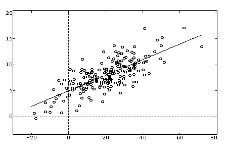
We fit the best curve, which can represent the relation between the x-y values. The equation of the curve is our required model of the relation between variables X and Y. Now, this curve can be linear or polynomial, forming the linear/polynomial regression respectively. It always depends on the data provided/observed (i.e. the training data) whether it produces a line or a curve. So, we have to form an equation of the relationship between X and Y and our job is done, the system will do the rest. Or will it?

Hypothesis
The equation we were talking about, let us call it our hypothesis equation. For linear regression, the equation will simply be the equation of a line, which can be written as,

Where ${\mathrm{\theta <!--THETA-->}}_0\text{,}{\mathrm{\theta <!--THETA-->}}_1$ are constants in the linear equation which can be represented by the vector $\mathrm{\theta <!--\; THETA\; -->}\text{ <!--NO-BREAK SPACE-->and <!--NO-BREAK SPACE-->}\mathrm{\epsilon \; <!--EPSILON-->}$ represents the error term.

If we assume the vector $X=\text{<}1,X\text{>}$ then we can also write the above equation in the form of multiplication of two vectors, as,

where ${\mathrm{\theta <!--THETA-->}}^{\mathrm{T}}$ is the transpose of $\mathrm{\theta <!--THETA-->}$.

This can be represented as a function (python language) :

def hypothesis(x,theta):

	tran = np.transpose(theta)
	z = np.dot(tran,x)
	#np.dot gives the dot product of two arrays.

	return z

The hypothesis is a simple representation of the regression model, but how do we attain this model or relation? Let us think about this. We have hundreds, maybe thousands of points on the graph, how would we fit the best line? The best line must have maximum number of points on itself. Also, the points which do not lie on the line, must be as close to the line as possible, in order to reduce the error percentage. This requires calculating the cost of the error each time we fit a line, and to minimise that error as much as possible. Next we study these two techniques.

Cost Function
We are going to understand how to calculate the cost. There can be two methods to do this. First, minimise the values of ${\mathrm{\theta <!--THETA-->}}_0\text{ <!--NO-BREAK SPACE-->and <!--NO-BREAK SPACE-->}{\mathrm{\theta <!--THETA-->}}_1$ so that the (predicted value - actual value) is minimized. The other could be the equation given below. In this, we are finding the distance between two points, the predicted point and the actual point, and we are attempting to minimise this distance. The distance is calculated using the Euclidean distance, but we ignore the square root (the values calculated might be small). The (2m) is only for ease of calculation.

This equation can be represented in python as:

def costFunction(theta,x,y):

	J = 0

	for i in range(m):

		yi = y[i:i+1]		#ith value
		xi = x[i:i+1]		#ith value
		hyp = hypothesis(xi,theta)

		a = np.subtract( hyp , yi )
		a = np.square( a )

		J += np.divide(a,2m)

	return J

The above equation represents the Cost Function. This cost function needs to be minimized in order for our regression line to be most effective. To minimise this function, we iteratively reduce the values of our $\mathrm{\theta <!--THETA-->}$ vector. How we do it, is explained next.

Gradient Descent
Gradient Descent is a universally used algorithm to iteratively arrive at the minimum of the cost function. Since we need to find the best line which fits each and every point on the graph, we need to change/update the values in our vector $\mathrm{\theta <!--THETA-->}$ so that they are minimum.

Let us first take a look at the cost function :

The differenciation of the function to find minimum, i.e.

which reduces to,

Now, we need to minimise our values of the vector $\mathrm{\theta <!--THETA-->}$, so we repeatedly reduce our vector values. The gradient descent function describes this by,

The above equation needs to be repeated till it converges in order to minimise.

Learning Rate ( $\mathrm{\alpha <!--ALPHA-->}$ )
The learning rate defines our step size. The step size can be any numerical value, but it has to be intelligently put. Consider this, if you take a large step size, you might reach a point on the curve when the $\mathrm{\theta <!--THETA-->}$ starts oscillating between two values and there is now way the process will converge. In such a case your machine will enter an infinite loop. If your step size is very small, the machine takes time to reach the minimum. So, the step size needs to be neither too large, nor too small, it has to be intelligently chosen with respect to your data.

Representing the above explanation as code:

def gradient_descent(theta,x,y,m):		# m is the number training records.
	
	alpha = 0.01
	diff = np.zeros(x.shape[1],dtype=float)

	for i in range(m):
		yi = y[i:i+1]
		xi = x[i:i+1]
		hyp = hypothesis(xi,theta)

		k = np.subtract( hyp, yi )
		diff = np.add(l, np.multiply( k, xi ))
		diff = np.multiply(alpha,l)

	theta = np.subtract(theta,l)

	return theta

The value of alpha I have taken above is random, but this value usually fits with most of the training data, since it is neither too large(2,3,5…) and nor is it too small(0.00001,0.0000002….).

Minimisation Function
The gradient descent needs to be repeatedly run untill convergence. This can be coded as:

def minimise(theta,x,y,m):		
	
	prevtheta = np.ones(x.shape[1],dtype=float)

	while prevtheta != theta:
		prevtheta = theta
		theta = gradient_descent(theta,x,y,m)
	
	return theta

Prediction
The prediction in linear regression is the hypothesis provided for the input values X. As you can see from the discussion above, when the $\mathrm{\theta <!--THETA-->}$ vector has been minimised, the output according to the machine will be the hypothesis produced by the linear regression equation that has been finally produced. That is, input vector X = < 1,x > multiplied by the new $\mathrm{\theta <!--THETA-->}$ vector, or,

Thus, the code for the output is:

import pandas as pd
import numpy as np

def main():

	X = pd.read_csv('train_input.csv')
	Y = pd.read_csv('train_output.csv')

	theta = np.ones(X.shape[1])
	m = X.shape[0]
	
	theta = minimise(theta,X,Y,m)
	
	INPUT = pd.read_csv('input.csv')

	OUTPUT = hypothesis(INPUT,theta)

	return OUTPUT